OTTO RÖSSLER

Otto Rössler
(photo from cccb.org)
Otto Rössler was born in Berlin, Germany in 1940. He obtained an M.D.degree in 1966 and became a researcher in theoretical biochemistry at the University of Tübingen (Germany).
Art Winfree, an American theoretical biologist, gave Rössler some copies of papers on the topic of chaos in 1975. These quickly got Otto interested in investigating chaos himself.
One year later Otto Rössler published a paper entitled “An Equation for Continuous Chaos” in which he modeled a chemical reaction using three simple nonlinear differential equations.
RÖSSLER’S EQUATIONS
dx/dt = -(y + z)
dy/dt = x + ay
dz/dt = b + xz – cz
where the three variables x, y, and z are functions of time and the values of the coefficients are a = 0.2, b = 0.2, c = 5.7
These Rössler equations are simpler than those Lorenz used since only one nonlinear term appears (the product xz in the third equation). Otto Rössler solved these equations on a computer. When he made a phase space diagram with the variables, he obtained what has become known as the “Rössler attractor.”
 Rössler Attractor
(from www.maplesoft.com)
You can click on the link below to read Rössler’s 1976 paper.
SIMULATING THE RÖSSLER EQUATIONS
Because three simultaneous equations are involved, with one of them being nonlinear, simulating the Rössler equations on LTspice is not a simple task unless you are an experienced LTspice user. However, help is available.
Glen Kleinschmidt in Australia has an excellent website ( glensstuff.com ) that deals with a variety of interesting topics. One of the things he discusses is simulating the Rössler equations and generating the Rössler attractor using LTspice.
Here’s a direct link to Glen’s page:
Glen even has an LTspice .asc circuit file that you can download and run to generate the Rössler attractor. I recommend that you visit his website and download his file. Read all of Glen’s comments CAREFULLY.
The strange attractor shown below was produced when I simulated the Rössler equations with LTspice using Glen’s .asc file.
 Glen’s Rössler Strange Attractor
(Click on the image to enlarge it.)
Glen used the “arbitrary behavioral voltage sources” available in LTspice to create the op-amps and the analog multiplier in his circuit. These are generic devices rather than components with a specific part number. They function very well when simulating chaotic circuits. However, these parts cause a circuit to behave slightly differently from how they would if specific components were used.
To demonstrate this, I created my own version of Glen’s circuit using LT1057 op-amps and the AD633 analog multi-plier. (In addition, I made a couple of other minor changes.) The Rössler strange attractor that I obtained from my circuit is shown below.
 My Rössler Strange Attractor
(Click on the image to enlarge it.)
You can see only slight differences between the two strange attractors. The differences are due entirely to using specific op-amps and a specific analog multiplier rather than generic ones configured from “arbitrary behavioral voltage sources.” The other minor changes I made had no effect on the strange attractor generated. This confirms what I said earlier that, in general, the chaotic circuits we are investigating are not particular about what op-amps are used.
The schematic circuit and the .asc file for my Rössler strange attractor circuit are available below.
 My_Rössler Schematic
(Click on the image to enlarge it.)
Remember that when you save this file you need to remove any .txt or other extension that is created so that you end up with the file name as MY_ROSSLER.asc
A Spice directive containing all the necessary information for the AD633 analog multiplier is contained on the circuit diagram. Also, since the LT1057 op-amp is part of the LTspice component library, you can run the simulation without worrying about adding additional components to LTspice.
To view the Rössler strange attractor after you have run the simulation, display V(vert) vs. V(horiz) from the “Visible Traces” option under “View” for the best display. You also can display any combination of V(x), V(y), or V(z) vs. one another.
Let me add that I obtained the LTspice model for the AD633 analog multiplier from the outstanding website (www.analog-innovations.com) by Jim Thompson. Jim did an excellent job of modifying the Spice model provided by Analog Devices to eliminate the convergence problems that were sometimes known to exist previously.
Below is a link to Jim Thompson’s website. Go to his “Device Models & Subcircuits” page if you want to download his model for the AD633. (This is only necessary if you plan to use the AD633 in your own circuits.) Check out all the other interesting things Jim has as well.
RÖSSLER’S HYPERCHAOTIC EQUATIONS
In 1979, Otto Rössler developed a set of four equations that described an autonomous “hyperchaotic” system.
The word “hyperchaotic” means that the system of equations must be at least four-dimensional (four variables). In addition, there must be two or more positive Lyapunov coefficients and the sum of all the Lyapunov coefficients must be negative.
The hyperchaotic set of equations that Rössler devised was:
dx/dt = -y -z
dy/dt = x + 0.25y + w
dz/dt = 3.0 + xz
dw/dt = -0.5z + 0.05w
Notice that the only nonlinearity is the xz term in the third equation.
Glen Kleinschmidt also has simulated Rössler’s hyperchaotic system. These files, too, are available on his website.
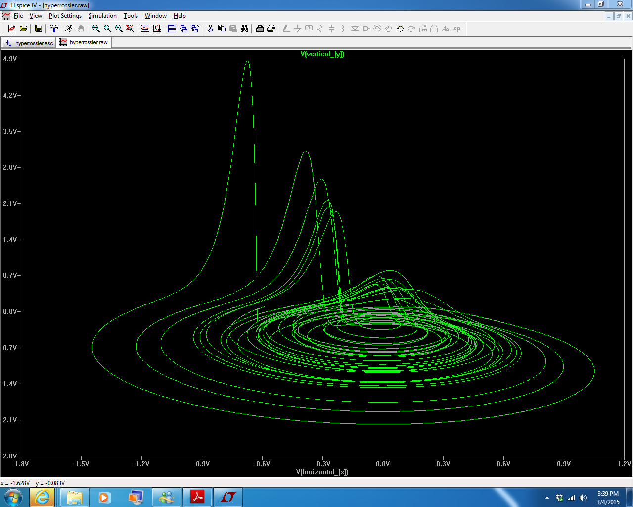
The Rössler hyperchaotic strange attractor I obtained when using Glen’s files with LTspice is shown below.

(Click on the image to enlarge it.)
AN IMPORTANT DIFFERENCE
It is important to note that when simulating or constructing Chau’s circuit, we are working with an actual oscillator electronic circuit. However, when dealing with the Rössler attractor, what we are simulating is an analog computer circuit which solves the Rössler equations.
There are numerous additional sets of chaos producing nonlinear differential equations that describe various other physical phenomena, rather than electronic circuits. Many of these sets of equations also can be solved by writing an analog computer program.
An analog computer program is really just an electronic circuit for solving differential equations. These circuits can be simulated using LTspice. Therefore, it is useful to take a little time to discuss analog computers. With a little practice, you, too, will be able to solve almost any set of chaotic equations using analog computer techniques.
ANALOG COMPUTERS
Analog computers were first developed in the 1930’s and were used during WWII to control such things as anti-aircraft guns on ships moving in rough seas. They were used extensively in the aerospace industry for many years (before digital computers became widely available) to solve both nonlinear as well as linear differential equations. Analog computer circuits still find many specialized uses today.
Operational amplifiers (or op-amps) are what make analog computers possible. Using op-amps, one can construct cir-cuits that perform the mathematical operations of algebraic sign reversal, addition, subtraction, multiplication, division, and also integration.
Those unfamiliar with analog computers but wishing to read an excellent introduction by Robert Paz describing how they work and are programmed are encouraged to click on the following link:
While analog computers lack the extreme accuracy and precision of digital computers, they are much easier to program. They also allow the user to change coefficient values quite simply. Analog computers, therefore, are ideal for solving many of the sets of nonlinear differential equations which describe chaotic phenomena.


